How to Create AI in Python: 9 Simple Steps To Know

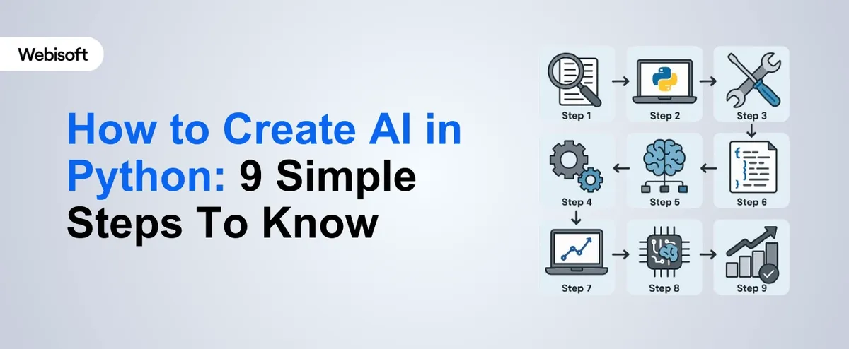
Python has become the standard for AI development because its ecosystem of libraries handles the heavy computational work, allowing you to focus on problem formulation and data quality. This guide covers the technical decisions that determine whether an AI project succeeds or fails.

Define the ML Task Precisely

Before writing code, map your business problem to a specific machine learning task. This determines your architecture, metrics, and test strategy.

• Classification: Predicting a discrete category (e.g., customer churn: yes/no). Use accuracy, precision, recall, and F1 score. Beware class imbalance (90% non-churn, 10% churn): accuracy alone is misleading.
• Regression: Predicting a continuous value (e.g., sales forecast). Use MAE or RMSE. Watch for outliers that inflate error metrics.
• Clustering: Grouping unlabeled data (e.g., customer segments). Silhouette score and Davies-Bouldin index validate grouping quality.
• NLP: Text classification, entity extraction, or generation. Requires tokenization, embedding, and sequence handling.

Misclassifying your task leads to wasted effort. A churn prediction built as regression instead of classification will perform poorly on business metrics.

Data Collection and Preprocessing

Data quality dominates model performance. A simple model on clean data outperforms a complex model on dirty data.

Data sourcing

• Transactional systems (SQL): Use SQLAlchemy to query directly into pandas DataFrames, avoiding manual exports.
• APIs: Use requests or httpx. Handle rate limiting (exponential backoff), pagination, and incomplete responses.
• Files: CSV, Parquet, or HDF5. Parquet is preferred for large datasets (column-oriented compression).

Preprocessing pipeline

Build preprocessing as a reusable sklearn.pipeline.Pipeline so training and inference use identical logic.

• Missing values: SimpleImputer fills with mean/median/forward-fill. Use the training set's statistic for test/production.
• Categorical encoding: OneHotEncoder for unordered (e.g., region), OrdinalEncoder for ordered (e.g., education level). Limit one-hot to <50 categories to avoid sparse matrices.
• Scaling: StandardScaler (mean=0, std=1) for normally distributed data. RobustScaler for data with outliers. Fit on training set only, apply to test.
• Feature engineering: Create new features from raw data (e.g., days-since-last-purchase). Domain knowledge beats random feature generation.

Train-test split: Use train_test_split with stratification for classification (maintains class distribution). Time-series data requires temporal split (no leakage from future to past).

Model Selection and Architecture

Choose based on interpretability needs, data size, and latency requirements.

Model Type	Pros	Cons	When to Use
Logistic Regression	Interpretable, fast, few hyperparameters	Assumes linear decision boundary	Baseline, regulatory requirements for interpretability
Random Forest	Handles non-linearity, feature importance built-in, robust to outliers	Slower inference, larger memory footprint, prone to overfitting	Tabular data, <1M rows, offline prediction
XGBoost	State-of-art on tabular data, feature importance, early stopping	Requires tuning, slow to train on large datasets	Competitive ML, kaggle-style problems
Neural Networks (TensorFlow/PyTorch)	Scales to large data, handles images/text, GPU acceleration	Requires more data (10k+ rows), black box, expensive to train	NLP, computer vision, very large datasets

Start with a baseline

Always train a simple model first (DummyClassifier, LogisticRegression, or RandomForestClassifier with default parameters). This establishes performance to beat and catches data issues early.

Training and Hyperparameter Tuning

Cross-validation

Use sklearn.model_selection.cross_val_score with StratifiedKFold (5-10 folds) to estimate true performance. Avoids overfitting to a single train-test split.

Hyperparameter tuning

• GridSearchCV: Exhaustive search over a parameter grid. Use when you have 2-3 hyperparameters and small search space.
• RandomizedSearchCV: Sample randomly from distributions. More efficient for large search spaces.
• Optuna: Bayesian optimization. Fastest for expensive-to-train models, learns which parameters matter most.

Monitor both training and validation loss to detect overfitting (training loss dropping while validation loss rises).

Evaluation and Validation

Metrics depend on the task. Use multiple metrics to avoid gaming a single one.

• Classification: Accuracy (overall correctness), Precision (false positives), Recall (false negatives), F1 (harmonic mean). Choose based on cost of errors. Missing fraud (low recall) is costly; approving fraudulent transactions (low precision) is also costly.
• Regression: MAE (mean absolute error, same units as target), RMSE (penalizes large errors), MAPE (percent error, useful for forecasting).

Use ConfusionMatrixDisplay and sklearn.metrics.classification_report to understand error patterns. A model with 95% accuracy but zero true positives is useless.

Production Deployment

Model serialization

Save the pipeline (preprocessing + model) as a single joblib or pickle file. Never reload code to preprocess; apply the saved pipeline.

Example (FastAPI):

from fastapi import FastAPI from joblib import load app = FastAPI() model = load('model.pkl') @app.post('/predict') async def predict(features: dict): prediction = model.predict([list(features.values())]) return {'prediction': float(prediction[0])}

Containerization

Docker ensures the same environment across development, testing, and production. Create a Dockerfile with Python, dependencies, and the saved model.

Monitoring

In production, track:

• Model performance: If actual outcomes diverge from predictions, model quality has degraded (data drift). Retrain weekly or monthly.
• Input distribution: Log feature statistics. If new data distribution differs significantly, model assumptions may be violated.
• Latency: Track prediction time. If it increases, infrastructure may be saturated.

Use MLflow, Weights & Biases, or cloud-native tools (AWS SageMaker, Google Vertex) to automate monitoring and retraining.

Common Pitfalls

Data leakage

Using information from the test set or future data during training. Example: normalizing the entire dataset before splitting (test set statistics influence training). Always fit preprocessing on training data only.

Overfitting

Model memorizes training data but fails on new data. Signs: training accuracy 99%, test accuracy 70%. Fix with regularization (L1/L2), dropout (deep learning), or simpler models.

Ignoring class imbalance

A 99% non-fraud dataset where you predict everything as non-fraud gets 99% accuracy but catches zero fraud. Use stratified splitting, class weighting, or oversampling minority class.

Insufficient data

Neural networks need 10k-1M rows. Tabular models need 1k+ rows per feature. Small datasets favor simpler models (logistic regression, Naive Bayes).

Essential Libraries

• pandas: Data loading, exploration, pivoting.
• NumPy: Numerical arrays and operations.
• scikit-learn: ML models, preprocessing, evaluation, cross-validation.
• TensorFlow/Keras or PyTorch: Deep learning. Keras (TensorFlow API) is simpler; PyTorch is more flexible for research.
• XGBoost or LightGBM: Gradient boosting (faster than sklearn).
• matplotlib/seaborn: Visualization and exploration.
• Jupyter Notebooks: Interactive development and documentation.

Workflow

A minimal production workflow:

1. Load and explore data (pandas, seaborn).
2. Build preprocessing pipeline (sklearn.pipeline).
3. Train baseline model (LogisticRegression or RandomForest).
4. Evaluate on test set (classification_report, confusion_matrix).
5. Tune hyperparameters if baseline underperforms (GridSearchCV or Optuna).
6. Iterate: improve features, try different models, analyze errors.
7. Save final pipeline and model (joblib).
8. Deploy to FastAPI + Docker or cloud platform.
9. Monitor predictions and input distribution monthly.
10. Retrain when performance degrades.

Summary

AI success in Python depends on clear problem formulation, data quality, and methodical evaluation. Use sklearn for tabular data and deep learning frameworks only when data scale or task complexity justifies it. Start simple, measure rigorously, and deploy with monitoring. The difference between a prototype and production is not the model, it's the infrastructure, monitoring, and retraining cadence.